Exploring Census Household Pulse Survey Part 1
Background
The Census Bureau began the Household Pulse Survey to measure the impacts of the Coronavirus Pandemic on the U.S. Household Population. This post will demonstrate some basics of downloading the data, getting it into R, and doing some simple analysis.
Download this post as an R Markdown file here.
Getting the data
This analysis will be based around using the Public Use File (PUF). The PUF contains the person-level responses to the survey and can be used to produce custom estimates. The PUFs for each week are published at https://www.census.gov/programs-surveys/household-pulse-survey/datasets.html.
The code below will download and unzip the data.
# icesTAF::mkdir("Data")
# download.file("https://www2.census.gov/programs-surveys/demo/datasets/hhp/2020/wk1/HPS_Week01_PUF_CSV.zip", "Data/HPS_Week01_PUF_CSV.zip")

# unzip("Data/HPS_Week01_PUF_CSV.zip", exdir = "Data/HPS_Week01_PUF_CSV")
Working with the data
library(forcats)
library(scales)
library(srvyr)
library(tidyverse)
First, we read in the PUF.
puf <- read_csv(file = "Data/HPS_Week01_PUF_CSV/pulse2020_puf_01.csv")The PUF contains the PWEIGHT variable to produce (weighted) estimates. In order to calculate standard errors though, we also need the “Replicate Weights” file, attaching it to the PUF.
repweights <- read_csv(file = "Data/HPS_Week01_PUF_CSV/pulse2020_repwgt_puf_01.csv")
puf_w_weights <- inner_join(puf, repweights, by = c("SCRAM","WEEK"))
Now, we convert data frame to survey object. This allows for calculating summary statistics without re-specifying the weight each time.
wgts <- colnames(repweights)[3:length(colnames(repweights))]

survey_puf <- as_survey_rep(puf_w_weights, id = SCRAM, weights = PWEIGHT,
                            repweights = all_of(wgts), type = "Fay", rho = 0.5005)
And now we should be all set to start analyzing the data. First, let’s make sure we know what we are doing by estimating something that already appears in the Detailed Tables. Specifically, we’ll look at the Housing 2b table. The table states that there are 8,918,242 persons in renter occupied housing units with No Confidence in the Ability to Pay Next Month’s Rent, 12,571,649 with slight confidence, and so on. We can replicate these numbers, adding the category IDs from the data.
renters_payment_confidence <-
survey_puf %>%
  filter(WEEK == "1" & TENURE == "3") %>%
  group_by(MORTCONF) %>%
  survey_count() %>%
  mutate_if(is.numeric, round, digits = 0)

renters_payment_confidence$MORTCONF <- factor(renters_payment_confidence$MORTCONF, labels =
                         c( "Question Seen But Category Not Collected",
                            "Missing / Did Not Report",
                            "No Confidence",
                            "Slight Confidence",
                            "Moderate Confidence",
                            "High Confidence",
                            "Payment Deferred"))

knitr::kable(renters_payment_confidence, format.args = list(big.mark = ","))| MORTCONF | n | n_se |
|---|---|---|
| Question Seen But Category Not Collected | 170,927 | 61,811 |
| Missing / Did Not Report | 153,139 | 37,374 |
| No Confidence | 8,918,242 | 377,552 |
| Slight Confidence | 12,571,649 | 374,676 |
| Moderate Confidence | 18,070,862 | 480,523 |
| High Confidence | 30,643,777 | 609,009 |
| Payment Deferred | 938,815 | 153,909 |
We see that we were able to successfully reproduce the estimates. However, the standard errors are slightly off. (If anyone knows why, please let me know.)
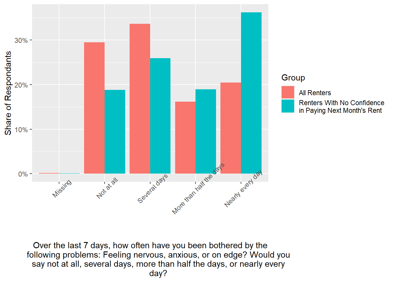
Now we can produce custom estimates. For example, the pulse asks respondents a series of questions about their mental health. Health Table 2a lists Symptoms of Anxiety By Selected Characteristics. However, the respondent’s housing situation is not one of the characteristics.
Let’s look at the symptoms of anxiety for renters.
anxiety_for_all_renters <- survey_puf %>%
  filter(WEEK == "1" & TENURE == "3") %>%
  group_by(ANXIOUS) %>%
  summarise(proportion = survey_mean())

anxiety_for_all_renters$Group <- "All Renters"

anxiety_for_renters_w_no_conf <- survey_puf %>%
  filter(  WEEK == "1" &
           TENURE == "3" &
           MORTCONF == "1" ) %>%
  group_by(ANXIOUS) %>%
  summarise(proportion = survey_mean())

anxiety_for_renters_w_no_conf$Group <- "Renters With No Confidence
in Paying Next Month's Rent"

anxiety_for_renters <- rbind(anxiety_for_all_renters, anxiety_for_renters_w_no_conf)

anxiety_for_renters$ANXIOUS <- factor(anxiety_for_renters$ANXIOUS, labels = c("Missing",
                                              "Not at all",
                                              "Several days",
                                              "More than half the days",
                                              "Nearly every day"))


ggplot(anxiety_for_renters, aes(x = ANXIOUS, y = proportion, fill = Group)) +
  geom_bar(stat = "identity", position = "dodge") +
  theme(axis.text.x = element_text(angle = 45)) +
  xlab("Over the last 7 days, how often have you been bothered by the
       following problems: Feeling nervous, anxious, or on edge? Would you
       say not at all, several days, more than half the days, or nearly every
       day?") +
  ylab("Share of Respondants") +
  scale_y_continuous(labels = scales::percent)
As might be expected, renters who report not being confident in their ability to pay next month’s rent also report feeling anxious more often.
One thing to note about the Pulse is that tenure (whether the home is owned or rented) is missing for a large number of the respondents.
tenure_w_missing <- survey_puf %>%
  filter(WEEK == "1") %>%
  group_by(TENURE) %>%
  summarise(proportion = survey_mean())
tenure_w_missing$TENURE <- factor(tenure_w_missing$TENURE, labels =
                         c( "Question Seen But Category Not Collected",
                            "Missing / Did Not Report",
                            "Owned free and clear",
                            "Owned with a mortgage",
                            "Rented",
                            "Occupied without payment of rent"))
tenure_w_missing$proportion <- scales::label_percent()(tenure_w_missing$proportion)

tenure_w_missing[,1:2]## # A tibble: 6 x 2
## TENURE proportion
## <fct> <chr>
## 1 Question Seen But Category Not Collected 0.5%
## 2 Missing / Did Not Report 10.2%
## 3 Owned free and clear 18.3%
## 4 Owned with a mortgage 40.8%
## 5 Rented 28.7%
## 6 Occupied without payment of rent 1.5%We can see from below that even though tenure is missing for a large share of respondants, the proportion of owners and renters appears in line with that reported in the American Community Survey.
tenure_no_missing <- survey_puf %>%
  filter(WEEK == "1" & TENURE != "-88" & TENURE != "-99") %>%
  group_by(TENURE) %>%
  summarise(proportion = survey_mean())

tenure_no_missing$TENURE <- factor(tenure_no_missing$TENURE, labels =
                         c( "Owned free and clear",
                            "Owned with a mortgage",
                            "Rented",
                            "Occupied without payment of rent"))
tenure_no_missing$proportion <- scales::label_percent()(tenure_no_missing$proportion)

tenure_no_missing[,1:2]## # A tibble: 4 x 2
## TENURE proportion
## <fct> <chr>
## 1 Owned free and clear 21%
## 2 Owned with a mortgage 46%
## 3 Rented 32%
## 4 Occupied without payment of rent 2%