Income vs. Rent Growth, Part 2
In the previous post, I looked at median gross rent and median household income growth from 2005 - 2023 according to the American Community Survey. But that analysis was only at the national level. What about the state level? Let’s find out.
Again, I’ll pull the median household income and median gross rent from the ACS. But this time I’ll select states. Additionally, I’ll switch to looking at median household income only for renter households. Finally, rather than looking at the full time series, I’ll only pull the starting and ending years.
state_hh_income <- get_ACS("NAME,B25119_003E","state",2005,2005,1)
state_hh_income2 <- get_ACS("B25119_003E","state",2023,2023,1)

state_hh_income$inc05 <- as.numeric(state_hh_income$B25119_003E)
state_hh_income2$inc23 <- as.numeric(state_hh_income2$B25119_003E)

state_hh_income <- cbind(state = state_hh_income$NAME,
                         inc05 = state_hh_income$inc05,
                         inc23 = state_hh_income2$inc23)

state_hh_income <- as_tibble(state_hh_income)

state_hh_income <- state_hh_income %>%
  mutate(inc_growth = as.numeric(inc23) / as.numeric(inc05) - 1)


state_hh_rent <- get_ACS("B25064_001E,NAME","state",2005,2005,1)
state_hh_rent2 <- get_ACS("B25064_001E","state",2023,2023,1)
state_hh_rent$rent05 <- as.numeric(state_hh_rent$B25064_001E)
state_hh_rent2$rent23 <- as.numeric(state_hh_rent2$B25064_001E)
state_hh_rent <- cbind(state = state_hh_rent$NAME,
                       rent05 = state_hh_rent$rent05,
                       rent23 = state_hh_rent2$rent23)
state_hh_rent <- as_tibble(state_hh_rent)
state_hh_rent <- state_hh_rent %>%
  mutate(rent_growth = as.numeric(rent23) / as.numeric(rent05) - 1
  )

state_income_rent <- merge(state_hh_income, state_hh_rent, by = "state")
state_income_rent <- state_income_rent %>%
  mutate(diff = rent_growth - inc_growth)

state_income_rent <- arrange(state_income_rent, desc(diff))
state_income_rent2 <- state_income_rent %>%
  select(state, inc_growth, rent_growth, diff) %>%
  mutate(across(c("inc_growth", "rent_growth", "diff"), function(x) (paste0(round(x, 4) * 100,"%"))))
States with the largest difference:
knitr::kable(head(state_income_rent2))| state | inc_growth | rent_growth | diff |
|---|---|---|---|
| Arizona | 90.42% | 124.27% | 33.85% |
| Florida | 81.34% | 112.48% | 31.14% |
| Hawaii | 66.36% | 94.97% | 28.62% |
| Delaware | 45.8% | 71.25% | 25.45% |
| Nevada | 63.83% | 88.39% | 24.56% |
| Wyoming | 61.81% | 86.22% | 24.41% |
Arizona and Florida had some of the fastest rent growth post-Covid, so this makes sense.
States with the smallest difference:
knitr::kable(tail(state_income_rent2))| state | inc_growth | rent_growth | diff | |
|---|---|---|---|---|
| 47 | Ohio | 74.57% | 65.42% | -9.15% |
| 48 | Puerto Rico | 55.94% | 46.58% | -9.37% |
| 49 | Vermont | 86.61% | 75.99% | -10.62% |
| 50 | West Virginia | 87.45% | 75.98% | -11.47% |
| 51 | Illinois | 80.26% | 68.66% | -11.59% |
| 52 | District of Columbia | 144.39% | 128.85% | -15.54% |
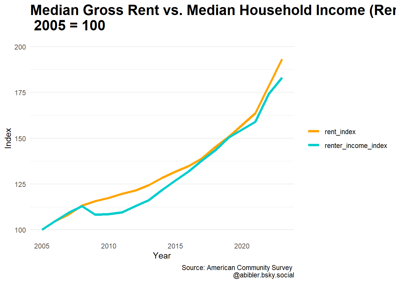
Let’s redo the national analysis, but this time with the renter median household income.
us_hh_income <- get_ACS("B25119_003E","us",2005,2019,1)
us_hh_income2 <- get_ACS("B25119_003E","us",2021,2023,1)
us_hh_income <- rbind(us_hh_income, us_hh_income2)

us_rent <- get_ACS("B25064_001E","us",2005,2019,1)
us_rent2 <- get_ACS("B25064_001E","us",2021,2023,1)
us_rent <- rbind(us_rent, us_rent2)

us_hh_income$B25119_003E[1]
## [1] "28251"us_hh_income <- us_hh_income %>%
mutate(income_index = as.numeric(B25119_003E) * 100 / 28251)
rent_start <- us_rent$B25064_001E[1]
us_rent <- us_rent %>%
mutate(rent_index = as.numeric(B25064_001E) * 100/ 728)
rent_income <- inner_join(us_hh_income, us_rent, by = "year")
rent_income$Difference <- rent_income$rent_index - rent_income$income_index
total_change <- rent_income %>%
select(rent_index, income_index, Difference)
total_change <- total_change[18,]
total_change2 <- total_change %>%
mutate(across(everything(), function(x) (paste0(round(x, 2),"%"))))
knitr::kable(total_change2)| rent_index | income_index | Difference |
|---|---|---|
| 193.13% | 183.07% | 10.06% |
df <- rent_income %>%
  select(year, rent_index, income_index) %>%
  rename(renter_income_index = income_index) %>%
  gather(key = "variable", value = "value", -year)


x <- ggplot(df, aes(x = year, y = value)) +
  geom_line(aes(color = variable), size = 1.5) +
  scale_color_manual(values = c("Orange", "cyan3")) +
  labs(caption = "Source: American Community Survey \n @abibler.bsky.social",
       title =
         "Median Gross Rent vs. Median Household Income (Renters), \n 2005 = 100") +
  ylab("Index") +
  xlab("Year") +
  theme_minimal() +
  scale_y_continuous(breaks=(seq(100, 200, 25)), limits = c(100, 200)) +
  theme(legend.title = element_blank(),
        panel.grid.major.x = element_blank(),
        panel.grid.minor.x = element_blank(),
        plot.title = element_text(size = 18, face = "bold"))
x
We can see that this time the difference is “only” 10%, and now the difference seems to be more due to the post-Covid rent spike.