Voucher Locations Part 1
Background
The Housing Choice Voucher program is the United States’s largest rental assistance program, providing rental subsidies to over 2.3 million households.
Location of Voucher Households
HUD provides geographic data on its assisted households in a variety of ways. HUD’s enterprise GIS service provides voucher locations by Census tract. HUD also provides data on Housing Choice Voucher households (and households in its other direct rental assistance programs) through an annual data set known as the ‘Picture of Subsidized Households.’ For this analysis we’ll look at the Picture data at the state level.
First we’ll want to set up our necessary packages.
# set libraries
library(httr)
library(readxl)
library(rjson)
library(tidycensus)
library(tidyverse)
library(tigris)
#
Next, we’ll download the Picture data.
# # Download Picture of Subsidized Household Data
# # icesTAF::mkdir("Data")
# # download.file("https://www.huduser.gov/portal/datasets/pictures/files/STATE_2023_2020census.xlsx", "Data/STATE_2023_2020census.xlsx", mode = "wb")
#
Then, we’ll read the data in to R and examine it.
#Read in picture data
state_picture <- read_excel("Data/STATE_2023_2020census.xlsx")

#Filter the data to only by the HCV program
vouchers_state <- state_picture %>% filter (program_label == "Housing Choice Vouchers")

#Look at states with the most and least vouchers
vouchers_state <- vouchers_state %>% arrange(desc(number_reported))
head(vouchers_state$States)
## [1] "CA California" "NY New York" "TX Texas" "FL Florida"
## [5] "IL Illinois" "MA Massachusetts"tail(vouchers_state$States)## [1] "DE Delaware" "AK Alaska"
## [3] "WY Wyoming" "GU Guam"
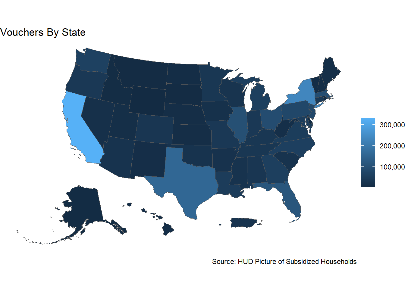
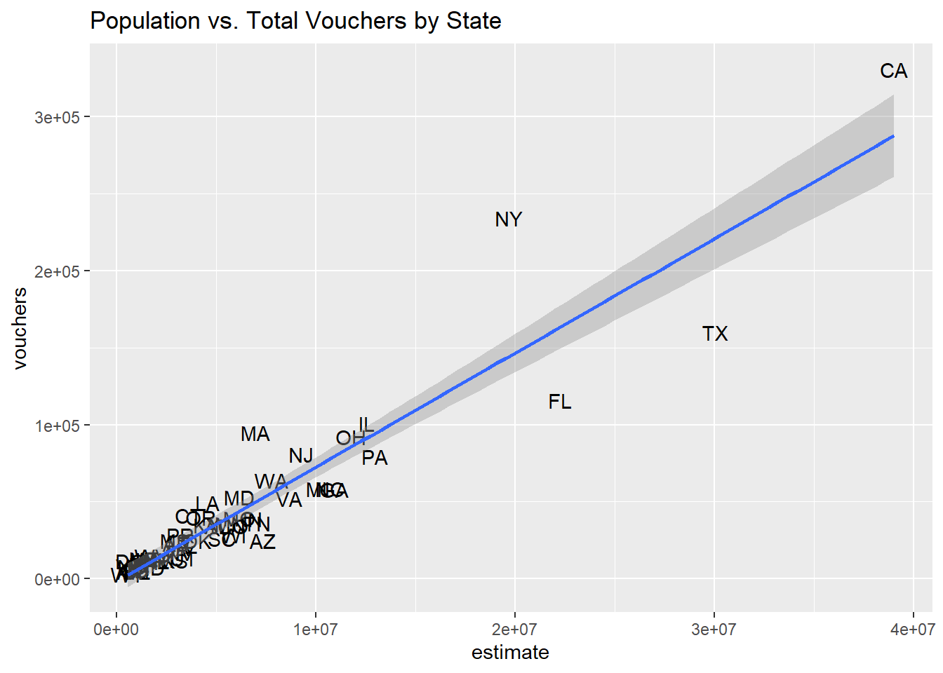
## [5] "VI U.S. Virgin Islands" "MP Northern Mariana Islands"Not surprisingly, California, New York, and Texas have the most voucher households as these states are the most populous. However, the relationship between vouchers and population isn’t quite perfect, as Texas (and Florida) actually have greater populations than New York. We can download population from the Census Bureau and attach it to the HUD data to examine this more closely.
# Get population from the ACS, using the tidycensus package, including a shapefile for mapping
state_population <- get_acs(
  geography = "state",
  variables = "B01003_001",
  year = 2022,
  survey = "acs1",
  geometry = TRUE,
  resolution = "20m"
) %>% shift_geometry()
# Attach the population the the Picture data
vouchers_pop <- inner_join(state_population, vouchers_state, by = c("GEOID" = "code"))
vouchers_pop <- vouchers_pop %>% rename(vouchers = number_reported)
# Plot the voucher data by state
ggplot(data = vouchers_pop, aes(fill = vouchers)) +
geom_sf() +
labs(title = "Vouchers By State",
caption = "Source: HUD Picture of Subsidized Households") +
scale_fill_continuous(name = "", label = scales::comma_format()) +
theme_void()
ggplot(vouchers_pop, aes(x=estimate, y=vouchers)) +
  geom_text(label = vouchers_pop$State) +
  geom_smooth(method=lm) +
  labs(title = "Population vs. Total Vouchers by State")
lmpop <- lm(vouchers ~ estimate, data = vouchers_pop)
summary(lmpop)
##
## Call:
## lm(formula = vouchers ~ estimate, data = vouchers_pop)
##
## Residuals:
## Min 1Q Median 3Q Max
## -60948 -8550 -155 5643 90054
##
## Coefficients:
## Estimate Std. Error t value Pr(>|t|)
## (Intercept) -1.868e+03 3.923e+03 -0.476 0.636
## estimate 7.420e-03 4.023e-04 18.444 <2e-16 ***
## ---
## Signif. codes: 0 '***' 0.001 '**' 0.01 '*' 0.05 '.' 0.1 ' ' 1
##
## Residual standard error: 21160 on 50 degrees of freedom
## Multiple R-squared: 0.8719, Adjusted R-squared: 0.8693
## F-statistic: 340.2 on 1 and 50 DF, p-value: < 2.2e-16Even though population explains about 87% of the variation in Vouchers by State, we see that New York and Massachusetts for example are overrepresented while stats like Texas and Florida are underrepresented.
Of course, Vouchers are not available to anyone but rather to low-income households. It is more likely that differences in low-income population sizes would explain differences in Voucher sizes better than overall population. We can get low-income population estimates from HUD’s Comprehensive Housing Affordability Strategy (CHAS) data.
# Read in the CHAS data
chas_states <- read_csv("Data\\CHAS\\2005thru2009-040-csv\\table1.csv")

#Calculate totals (Adding renters with and without conditions)
chas_states <-  chas_states %>% mutate(
  fips = substr(geoid, 8, 9),
  Total_HHs_LE_30pct = T1_est77 + T1_est113,
  Total_HHs_LE_30pct_moe = (T1_moe77^2 + T1_moe113^2)^.5,
  Share_HHs_LE_30pct = Total_HHs_LE_30pct / T1_est75,
  Total_HHs_LE_50pct = Total_HHs_LE_30pct + T1_est84 + T1_est120,
  Total_HHs_LE_50pct_moe = (Total_HHs_LE_30pct_moe^2 + T1_moe84^2 + T1_moe120^2)^.5,
  Share_HHs_LE_50pct = Total_HHs_LE_50pct / T1_est75,
  Share_HHs_LE_50pct_moe = Total_HHs_LE_50pct_moe / T1_est1,
  Total_HHs_LE_80pct = Total_HHs_LE_50pct + T1_est91 + T1_est127,
  Share_HHs_LE_80pct = Total_HHs_LE_80pct / T1_est75)

# Attache the CHAS data to the population and Voucher data
pop_program <- inner_join(vouchers_pop, chas_states, by = c("GEOID" = "ST"))

lm_vli <- lm(vouchers ~ Total_HHs_LE_80pct, data = pop_program)
summary(lm_vli)
##
## Call:
## lm(formula = vouchers ~ Total_HHs_LE_80pct, data = pop_program)
##
## Residuals:
## Min 1Q Median 3Q Max
## -41785 -9400 1133 7250 66621
##
## Coefficients:
## Estimate Std. Error t value Pr(>|t|)
## (Intercept) -6.276e+03 3.644e+03 -1.722 0.0912 .
## Total_HHs_LE_80pct 4.800e-02 2.305e-03 20.826 <2e-16 ***
## ---
## Signif. codes: 0 '***' 0.001 '**' 0.01 '*' 0.05 '.' 0.1 ' ' 1
##
## Residual standard error: 19000 on 50 degrees of freedom
## Multiple R-squared: 0.8966, Adjusted R-squared: 0.8946
## F-statistic: 433.7 on 1 and 50 DF, p-value: < 2.2e-16#Plot the relationship
ggplot(pop_program, aes(x=Total_HHs_LE_80pct, y=vouchers)) +
geom_text(label = vouchers_pop$State) +
geom_smooth(method=lm) +
labs(title = "Low Income Population vs. Total Vouchers by State")
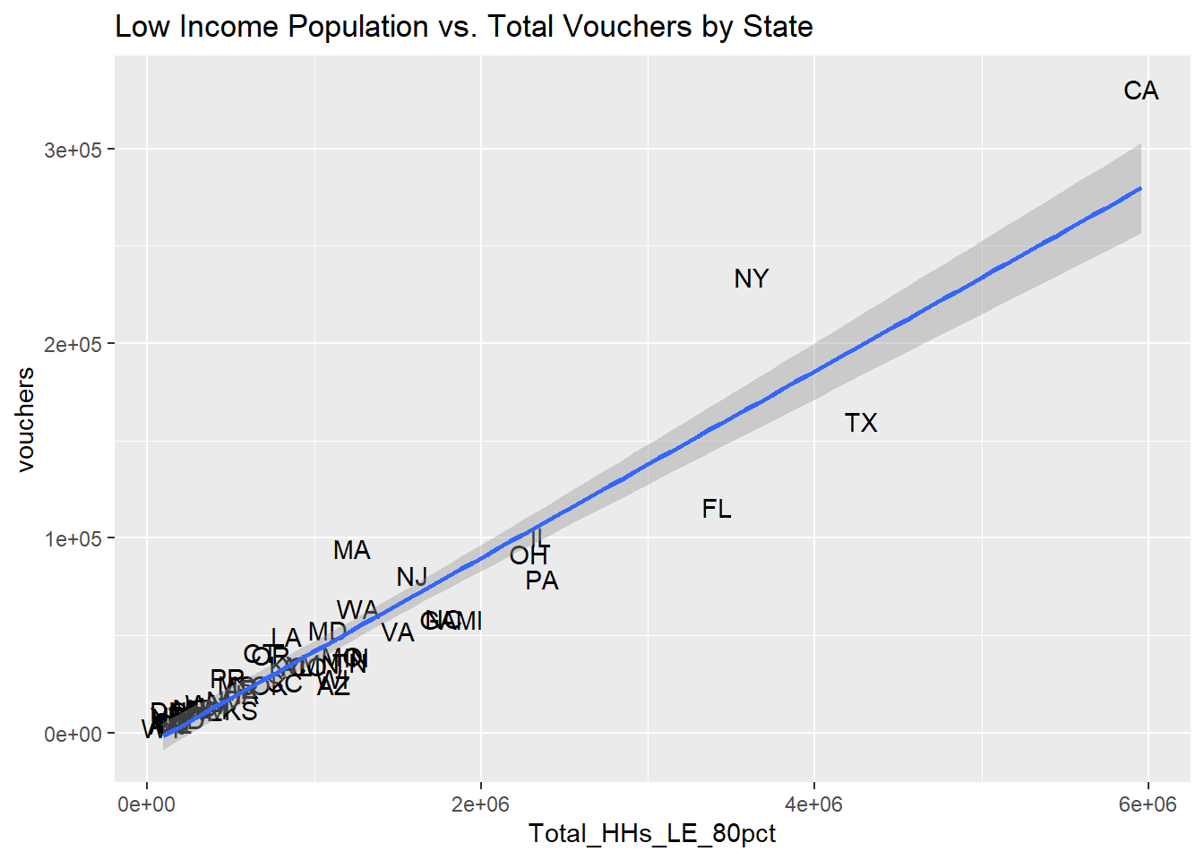
It turns out that low-income renter population explains the variation in state vouchers only modestly more than overall population.
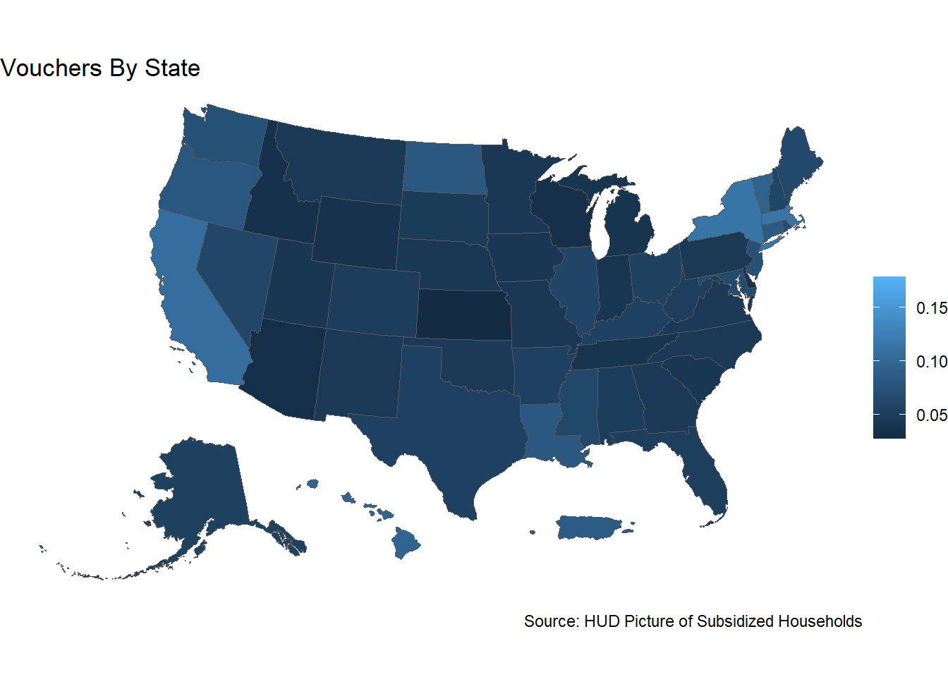
We can also look at the share of the very low-income population receiving vouchers by state.
pop_program <- pop_program %>% mutate(voucher_share_VLI = vouchers / Total_HHs_LE_50pct)

ggplot(data = pop_program, aes(fill = voucher_share_VLI)) +
  geom_sf() +
  labs(title = "Vouchers By State",
       caption = "Source: HUD Picture of Subsidized Households") +
  scale_fill_continuous(name = "", label = scales::comma_format()) +
  theme_void()
summary(pop_program$voucher_share_VLI)## Min. 1st Qu. Median Mean 3rd Qu. Max.
## 0.02770 0.04459 0.05174 0.06100 0.07199 0.17931